
From Kevin Bacon to HNSW: the intuition behind semantic search and vector databases
In this 3-part series, I deep dive into vector search and ANN indexing, the limitations of scaling popular algorithms like HNSW, and how I built an open source vector DB for querying across billions of vectors on commodity machines, called CoreNN. For example, here it is searching across 1 billion Reddit comment embeddings in 15 ms from a 4.8 TB index on disk—all time is spent embedding the query and fetching results:
A brief primer: vectors, like neural embeddings, can be used to represent anything, often text and images. This can be used for search, where the closest vector to a query is the best matching result. The problem of finding the nearest candidate vector to a query vector is known as nearest neighbor search. You can read more about semantic search and AI embeddings in this post.
Productionizing this retrieval system requires a mechanism to perform this with high accuracy and low latency. The naive way is to compare the query to every candidate, which is O(n); algorithms exist to build indices for searching vectors in O(log n) time, such as HNSW. In this first post of the series, I'll provide an explanation on how ANN search works, why it's able to achieve high recall in sublinear time, and the context and intuition behind the graph algorithms and data structures that power them, including HNSW, with interactive demos.
Don't miss the other posts in this series:
- From Kevin Bacon to HNSW: the intuition behind semantic search and vector databases
- From 3 TB RAM to 96 GB: superseding billion vector HNSW with 40x cheaper DiskANN
- Building a high recall vector database serving 1 billion embeddings from a single machine
- Curse of dimensionality
- Graphs
- Six Degrees of Kevin Bacon
- Hierarchical Navigable Small World (HNSW)
- DiskANN
Curse of dimensionality
Our goal is to be able to find the closest k vectors in sublinear time, as doing a brute-force scan is not efficient enough for most use cases. There are many use cases for this, not just modern neural embeddings. Essentially, we want some ideal data structure to index vectors.
Existing data structures like k-d trees and locality-sensitive hashing exist, but they tend to degrade to O(n) time complexity in higher-dimensional spaces due to the curse of dimensionality. This is described better by many others: empirical, formal analysis, geometric, probabilistic. I will attempt to explain in a more informal way.
The main issue is distances becoming uniformly far and therefore less discriminating. I discovered some interesting intuitions to think about this:
-
Imagine a 2D shape, like a circle. As you move from the center to the periphery, a few points get closer, but more points get further away. As dimensions increase, the space of this periphery dominates and the "center" is vanishingly small (see this great visualization). Most points will lie "near the edge", and the expansive volume means almost every other point is near some other edge (unlikely to be near the exact same place or the tiny center), so almost everything's uniformly (edge A <-> center <-> edge B) far (edge to edge) away from everything else, including the "nearest" neighbors.
-
Given a point as a vector, being near the edge only requires one element being near the min/max for that element – imagine a 2D square with (x, y) points (vectors) and see this is true. Given many elements, it's very unlikely for a point to be "in the center", where every single element happens to be near its mean. This is why most points are "near the edge" in high dimensional space. The more contributing dimensions to the difference between two vectors, the higher the mean distance (distances are far) and lower the variance (distances are uniform); exceptions are usually due to skewed data or non-independent features.
A more relatable real-world example: we could model humans as a vector of trait probabilities. Humans are complex, so there may be thousands of features.
- People are unlikely to be "perfectly normal", where every dimension is average; we're all "near the boundary" in this high-dimensional space.
- Person A can be similar to B because of traits 1, C by 2+3, D by 1+4+5, and so on. It's hard to cleanly delineate the search space and organize people in a rigid hierarchy or groups.
I'd recommend going through the interesting links above if you're interested. They provide more context and background, different perspectives and intuitions, and more thorough explanations for what the curse is, what happens, and why it matters.
Because these data structures rely on distances to prune the search space quickly, but distances become less useful in higher dimensions, they don't work well in practice.
Graphs
This curse led to the discovery of graphs as the ideal data structure. We can model the problem as a graph by making searchable vectors (e.g. documents) nodes, and query by traversing the graph to find the node with the minimum distance to the query, representing our nearest neighbor. Unlike trees and hashes, we have a lot of flexibility, as edges can connect any two nodes (vectors); for example, we can connect two vectors simply because they're close – no need to find some ideal partition or hash function.
The graph should be greedily traversable such that, starting from some fixed entry node, we can stop when we've reached a local minima and be confident that it is the true neighbor. Otherwise, we can always say "the true neighbor could be elsewhere" and end up doing a global search, defeating the purpose.
The flexibility of graphs is what makes them work over the others: we can "adapt" the graph to our data distribution (whatever it is) and our greedy "query" operation, to ensure sublinear time complexity (i.e. not global search) regardless of our data.
Now we have an optimization problem: what edges should we pick to optimize for these outcomes?
A random graph – where every node has N arbitrary edges to other nodes – is a good baseline to establish the lower bound of effectiveness, and why smarter approaches discussed later are necessary. Let's try that:
The above is an interactive visualization. Vectors here are 2D (represented via positioned dots) for easy human visualization, and lines are the random edges. The blue node is the randomly-picked entry node, and the purple node is your query. Try it a few times: click anywhere to query that position, and the path taken to find it (or fail to) will light up.
After a few times, you'll notice that many queries fail to find the ground truth (the true nearest neighbor i.e. k=1), and that they take zig-zagged inefficient paths. This gets worse with more data points and higher-dimensional spaces – many queries succeed here by "luck", as the space is small and points are few.
This indicates we need to add some structure to this graph, as pure randomness doesn't work. So how do we figure out what this structure should be?
Six Degrees of Kevin Bacon
It turns out sociology can help us. HNSW has its roots from the famous Milgram small-world experiment ("six degrees of separation"), which found that most people can be reached from anyone else using only about six "short paths"—who each person knows personally—instead of having to know everyone else. Another way to see this is that the average path between any two people is logarithmic (i.e. sublinear) to the population.
Our needs are similar: we have a graph, with potentially billions of nodes, and we'd like to get to some specific node (the closest to some query) from some starting node. So what can we glean from how our society works?
- Our transportation is designed hierarchically, with long (highways), medium (avenues), and short (streets) mechanisms for getting anywhere without connecting every possible two points.
- In the Milgram experiment, people forwarded the letters to distant strangers by first giving to long-range connections (people who could bridge social groups, geographies, etc.), then to more local connections.
Long connections makes short work to get to the "general" area, which we then use short connections to hone in on the "neighborhood" for accuracy. And there's no global knowledge–we simply go to our nearest connection and navigate from there. If we translate to our desired graph properties:
- We'd like an ideal distribution of long edges such that we can get to where we need quickly, preferably in sublinear time.
- The edges should be picked optimally in such a way that we can find the global optima only by traversing the locally nearest adjacent nodes, so we can stop in sublinear time.
Armed with this knowledge, let's try some smarter strategies for placing edges. Let's start with the most simple idea: use some ratio of short to long edges.
To explore this idea, I've extended the demo to allow tweaking how many edges should connect to nearby nodes (short edges) and how many should be random (likely long edges, given most nodes are definitionally relatively further away). Play around with the parameters and get a sense for what works well.
In general, adding structure by connecting neighbors increases accuracy, up to a point, before local minimas prevent reachability too often (and the paths are inefficient with too many hops). There's also a relationship between node count and edge count, which we'll analyze deeper later. So it's on the right track, but we need to more explicitly figure out how to pick optimal edges rather than just guessing the ratio and picking random edges.
There's a great post by Bartholomy for further reading on the sociology context and structure behind ANN graphs.
Hierarchical Navigable Small World (HNSW)
While CoreNN doesn't use HNSW, it is the current most-popular graph-based ANN index and forerunner to the Vamana algorithm CoreNN uses.
It's interesting to think about how to add those long edges strategically such that they empirically allow quick navigation across the graph regardless of the destination. HNSW's innovation is the H in its name. We can build a graph by inserting edges to neighbors of each node; once we are in the "neighborhood", this should allow us to find our exact target with a few hops. This also makes edge selection simple: just connect to the closest nodes. However, as previously mentioned, we also need some long edges. The HNSW authors came up with a neat trick to build on top of this to get optimal long edges without much extra effort:
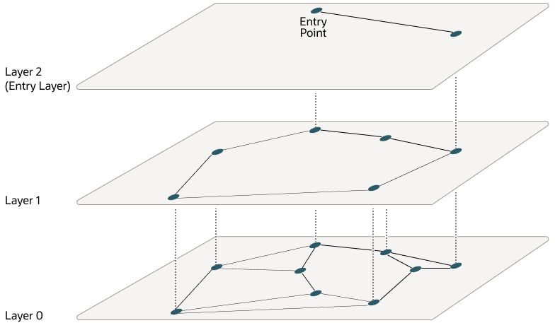
We can build multiple graphs called levels, where each higher level has uniformly-sampled fewer nodes, and the bottom level is our graph of all nodes. When building, we use the same approach to each level graph for picking edges, but a node is randomly assigned to a specific level (the higher, the less likely) and inserted to that level + all below it.
Why does this work? Think about how uniform sampling works: we pick nodes from across the map, but there are much fewer at a higher level. Now, edges are longer on average, because it's unlikely that a node's true neighbor also happens to be at the same level, so its level-specific neighbors are likely further away and "spread" across the map. We're still just adding edges based on nearest neighbors. It's easier to see in the visualization above: just by reducing the amount of nodes at a higher level, we get longer edges as a result.
Now we can navigate quickly: starting from the top-most level, we find the nearest node to our query. Then we drop down to the level below at the same node, and repeat. Long edges at the higher levels navigate quickly; shorter ones below hone in on the exact local neighborhood.
It's important to note that we're not intentionally picking spread-out nodes. It's still uniform sampling, so the data distribution is still the same. This is important, as we want our graph to be optimized for our dataset. If there are 100 nodes spread out across the latent space, but 1,000 in this one small corner, we want our higher levels to have more nodes in that small corner too. While they don't help queries "jump far" in absolute distances, they still skip over large amounts of nodes, helping navigate that dense region. If we intentionally only pick one node from that entire area for the higher level, we'd have to explore 1,000 once we drop down.
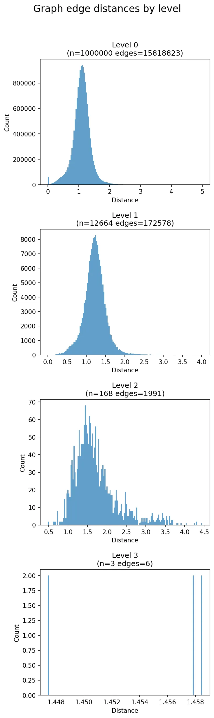
HNSW uses an exponential decay for the probability of being picked in each successive level. As you'd expect, this means that each level has exponentially fewer nodes than the one below it. It's logarithmic because we want to have sublinear querying time, so this way, we exponentially "close the gap" to our target at each level. You can think of it as similar to narrowing the "cone of visibility" each time.
Empirically, this works extremely well in terms of query accuracy and speed, which is why HNSW is still popular. For more details on how HNSW works, see this great article by Oracle.
DiskANN
In the next post, I'll go into the limitations of HNSW, why it's hard to use HNSW at scale in practice, and dive deep into DiskANN, an approach that improves upon the graph algorithms to make them work effectively from disk rather than expensive RAM, reducing costs by 40x and enabling far greater scalability.