
From 3 TB RAM to 96 GB: superseding billion vector HNSW with 40x cheaper DiskANN
In this 3-part series, I deep dive into vector search and ANN indexing, the limitations of scaling popular algorithms like HNSW, and how I built an open source vector DB for querying across billions of vectors on commodity machines, called CoreNN. For example, here it is searching across 1 billion Reddit comment embeddings in 15 ms from a 4.8 TB index on disk—all time is spent embedding the query and fetching results:
In the previous post, I provide an introduction and explanation to the problem of searching across vectors (like neural embeddings) efficiently, and the intuition and theory behind why graph-based algorithms like HNSW solve the problem. In this post, I'll go into the limitations of HNSW that make it difficult to use in production systems at scale, and dive deep into DiskANN, an approach that leverages the high recall and flexibility of graphs while making them disk-native, making it possible to cost effectively serve and query billion-scale indices of embeddings.
DiskANN serves as the foundation for CoreNN, which allowed me to scale down my web search engine cluster of sharded HNSW indices totalling 3 TB RAM into a single 96 GB RAM machine, reducing upkeep cost and operational burden. This post dives into DiskANN, while the next post focuses on CoreNN.
Don't miss the other posts in this series:
- From Kevin Bacon to HNSW: the intuition behind semantic search and vector databases
- From 3 TB RAM to 96 GB: superseding billion vector HNSW with 40x cheaper DiskANN
- Building a high recall vector database serving 1 billion embeddings from a single machine
Limitations of HNSW
As discovered in the last post, HNSW works well for high recall vector search in sublinear time, suitable for low latency querying over large scale indices, which my web search engine required.
CoreNN didn't exist yet at the time I was working on my search engine, so HNSW was my pick. However, HNSW has some limitations for large-scale indices:
Memory access assumption
The algorithm was designed with memory operations in mind, and trying to use it from disk is too slow.
It takes around 100 ns to read memory, and 20,000 ns to read a random 4K SSD page. This is a 200x increase — differences of this magnitude break the assumptions that algorithms build around; one could perform multiple queries from in-memory HNSW before even a single node read request returns.
Its design also means that the index must be loaded entirely into memory before you can use it, even for just a few queries. Even some vector databases have this requirement.
If you have more vectors than you can fit in memory, you now have to shard your indices so you can use multiple machines for more combined memory. As I scaled my search engine, I ended up running a cluster of expensive high-memory machines with a combined 3 TB of RAM, which wasn't cost-efficient.
True deletions
The algorithm, as described in the original paper, was not designed with a mechanism to truly delete vectors. There are some discussions on possible approaches, but as of right now the official hnswlib library still has no such API.
Deletions are currently handled by marking them as deleted in the graph, and filtering them out in the final results. This poses a problem: as more and more nodes are deleted, more and more of the graph is "garbage" and queries waste a lot of time visiting them only to discard them.
Note that updates are also deletes; you can't simply change the vector of a node, or delete it from the graph, because the graph edges are optimally picked in order to make it navigable with that node as it exists.
Storage format
hnswlib, the official library, saves and loads the index essentially using memory dumps. While fast and simple, this makes it hard to do updates and persist them without a full rewrite. Given how large indices can be, this can become problematic. For example, inserting 10 vectors (<1 MB) into a 250 GB index requires copying the file to a large machine, loading into memory, performing the insert, then dumping 250 GB back to disk.
Vamana
In 2019, Microsoft Research published a paper: high accuracy, low latency querying over 1B embeddings on a 64 GB machine, by leveraging the disk. It defines a new graph, Vamana, with a new strategy, DiskANN, for using the disk with it. Combined, they bring a few innovations over HNSW:
- Simpler algorithms for querying and inserting that only need one graph, building optimal long edges without the need of a hierarchy.
- Tunable parameter to create longer edges, which allows fewer hops to navigate to the "local" area (and therefore fewer disk reads).
- A procedure for truly deleting vectors in a disk-efficient manner.
- An optimized storage layout and querying approach that exploit SSD characteristics — and allows indices to be queried from much larger and cheaper SSDs while retaining high accuracy.
It's a graph algorithm, in the same vein as HNSW, so it works via two mechanisms:
- Search: repeatedly expand the closest unvisited node in the search list (starting from the entry node) by inserting its neighbors into the search list. Stop once there are no more unvisited nodes.
- Insert: query the vector to insert (I) and collect all the nodes we visit (V) along the way. Insert edges V→I and I→V, except for any V where it's greedier to go V→V'→I.
Intuitively, we can see that the search is greedy and only considers the local optima. We can also see that the insert works by making it easier to reach I next time simply by adding all edges we saw on our path. It'll create long edges from the earlier nodes in V, short edges from the final nodes we saw before we found I, and everything in between. Where HNSW has to add another mechanism (hierarchy) to get those longer edges, Vamana doesn't. Nice and simple.
Because V can be quite large, and backedges are also inserted to the nodes on the other end, nodes can exceed the degree bound (the limit of edges a node can have, akin to M in HNSW). The degree bound is important to avoid excessive disk reads (i.e. tail latencies). RobustPrune is Vamana's innovation for ensuring this while still picking edges that result in a high quality graph.
One thing it does: we don't need V→I if V'→I exists and V is closer to V' than I. This is because our algorithm is greedy, so at V we'll go to V' (or some other node) and from there find I. One cool thing is that we don't actually check if V→I exists, the built graph just ends up making this work—no locking and consistency complexity necessary.
But what about long edges? HNSW had the hierarchy, but Vamana doesn't, so just picking the closest neighbors won't work as we saw from that earlier experiment.
RobustPrune therefore also has an alpha parameter, where alpha >= 1.0: instead of pruning all V→I where there is another greedier indirect path, we give some additional slack by setting the threshold to be (V → I) <= (V → V') * alpha, allowing some longer paths to survive. Note that alpha = 1 means we're back to no slack. This might be easier to see:
Blue edges are the candidates for connecting to the target node. All nodes we visit are candidates for one end. Notice how rarely we pick longer edges, with the edge from the entry point being the most obvious, unless we increase alpha, which allows us to tune based on what works best for our data distribution.
Combined, these pick and remove edges in a more intelligent way that enforces the hard upper bound limit of edges, while also preserving only the best edges that result in a high quality graph.
Deletion works in a similar fashion: we can't simply "delete" a node as its edges are part of the network for effective navigating, so the simplest approach is to connect all nodes connected to it to all nodes it connects to (a.k.a. contraction). However, this adds a lot of extra edges, likely redundant and exceeding the limit. Because we have RobustPrune, we can handle this by running that on all affected nodes. This allows for true deletions while preserving the quality of the network.
Let's now implement Vamana in our interactive demo to see that it works and how it compares to our strategies so far:
Analyzing Vamana
Let's empirically investigate how well Vamana works and what effects its parameters have. We'll use the popular GIST1M dataset, as it's reasonably large (1M) and high dimensional (960).
To greatly speed up exploring the space of hyperparameters, I precomputed the pairwise distance between all vectors in batches on a GPU using a small Python script. RobustPrune does O(n2) comparisons, so this reduces the time to build and evaluate each index configuration. The dataset was subsampled to 250K as 1M×1M f16 requires 1.8 TB of RAM. (Reading from slow disk in order to avoid much faster CPU computation defeats the purpose.)
We know there's a parameter for how many edges each node should have. The higher this is, the better steps we take at each hop, with the trade-off being that we must compare the query against every edge (so the more edges, the more computation). It's easy to see this if we take the extremes:
- If a node has edges to every single other node, we can take the perfect step by going straight to our target node, at the cost of doing essentially a brute force global scan.
- If a node has only one edge, it's unlikely that we'll take a good step in the direction and distance we want—what are the chances that our query just happens to align with that edge?
The curse of dimensionality applies: as higher dimensions means more disparate vectors are similar, we need more edges for better disambiguation. It's also the reason why we have to check every edge: very different vectors can be similar, and we can't cleanly divide the space. Let's take a look at various values for this parameter:
Here, we use the HNSW notation and refer to the degree bound as M. (You can also see the effects of different alpha parameter values via the top dropdown, discussed next.) The chart shows how quickly it found the true neighbors for queries on average, and there's a clear trend: the higher the M, the more accurate and quickly-converging. We can also see the sublinear characteristics generally: queries rapidly converge (thanks to those long edges) and we find most neighbors in just a few iterations, with diminishing returns as we try to find every last neighbor. In our high-dimensional space, we can clearly get more gains as we increase M until around 150. In fact, there appears to be an optimal minimum; below M=32, queries are not only inaccurate, but also take a lot longer to complete.
To put it simply: higher M = better accuracy, with diminishing returns past a certain point. Increase by as much query compute time you're willing to pay, and don't drop below a certain point.
The other main parameter is alpha, which increases the preservation of longer edges during the RobustPrune algorithm. If we transpose the chart and instead compare alpha values given a reasonable M:
To make it easier to see, it only highlights 4 values initially: 1.0, 1.1, 1.2, and 4.0. (Click legend items to toggle them.) Compared to M, it's more interesting, as there isn't a clear relationship between increasing alpha and increasing accuracy. It peaks at around 1.1, before dropping quite dramatically. It seems that excessive long edges forced a suboptimal graph fit for our dataset, and after alpha=1.1 they hinder instead of help query hops on average. This shows the importance of evals for quantifying effects of changing hyperparameters for your dataset.
We can take a look at the graph and query properties to see some of the internals as we tweak these hyperparameters. Let's start with the basic one: does alpha change edge lengths? If we look at the distribution of edge lengths, we can see that increasing alpha not only increases long edges, but all edges across the board:
This is expected as the alpha parameter increases acceptable edge lengths during pruning, so more edges are kept overall. Keep this in mind as we go through the subsequent analyses.
Let's look at the distance of the next closest node to expand at each query iteration:
We can see that the graph was very well optimized, and we rapidly closed in on the local neighborhood, and then spent a long time in the neighborhood to find every last neighbor. Our most optimized variant closed in the quickest.
Another perspective, told in two charts:
In the first chart, we can see that all the top-performing parameters make efficient graphs, where most nodes newly discovered are not discarded due to being seen before. In the second chart, even amongst the top-performing alpha values, alpha=1.1 stands out, by dropping the fewest newly discovered nodes, with a noticeable difference to the other high performers; it's the most efficient amongst the most accurate.
Meanwhile, we see the issues with the "unconverging" low alpha values not finding many nodes and exploiting the graph enough. On the other hand, the high alpha values are finding lots of candidate nodes but dropping most of them, likely "overconverging" and unable to hone in accurately in the local area.
Comparison between HNSW and Vamana
Because both HNSW and Vamana both build graphs with similar goals and properties (e.g. greedily searchable, sparse neighborhood graphs), I suspected it was possible to leverage CoreNN over existing HNSW indices, which I had and wanted to migrate without expensive rebuilds. To verify this, I analyzed the graphs that Vamana and HNSW build. To make HNSW graphs comparable to Vamana, I flattened all levels into one graph, merging all edges across all levels for each given node.
When looking at the graph edge distribution when built over the GIST1M dataset with the same parameters, we see a similar shape:
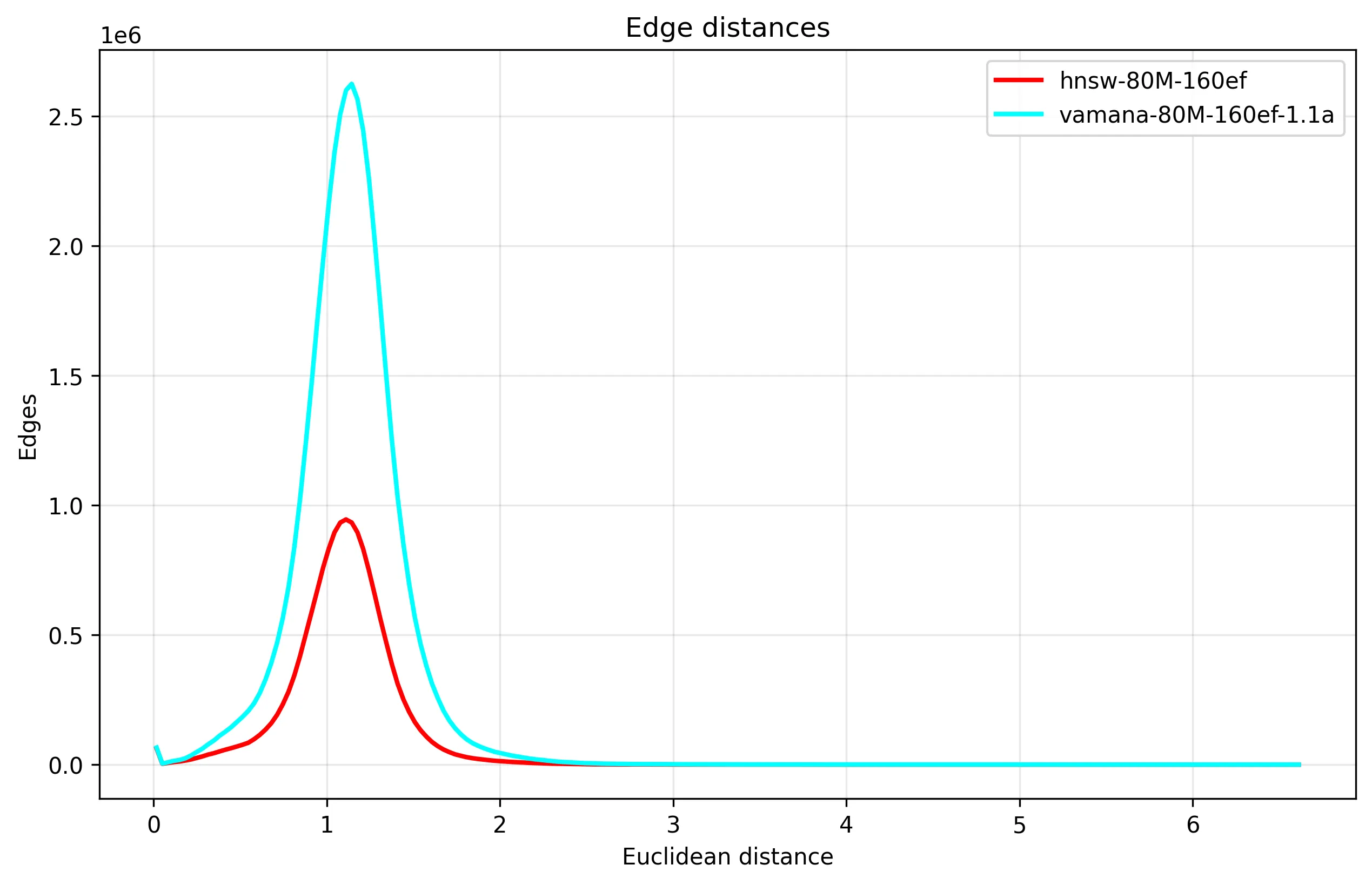
From this, we can see that the Vamana graph has a lot more edges, which we can confirm from the distribution of node edge counts, where Vamana is utilizing the degree bound a lot more:
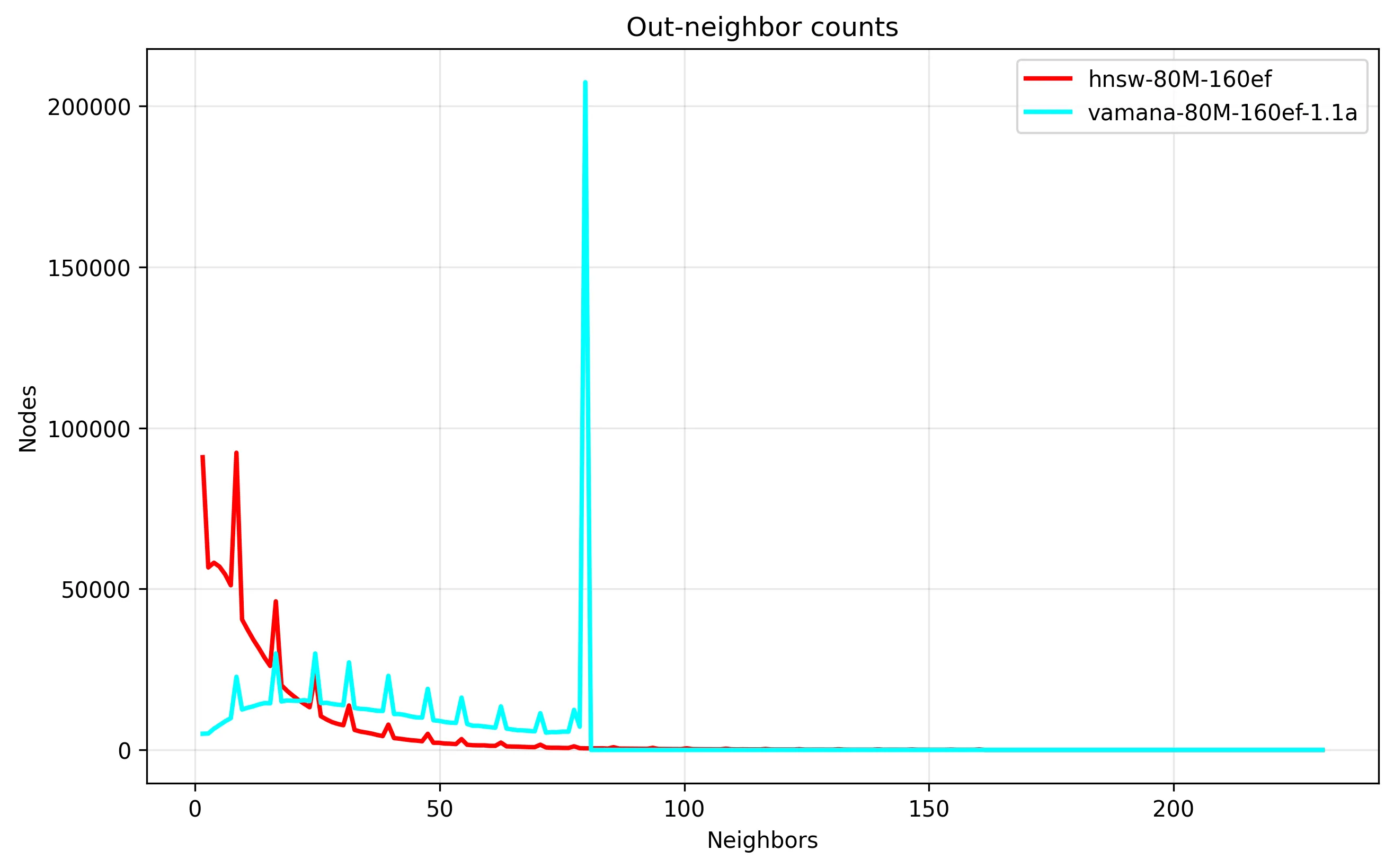
We also see that Vamana enforces a strict upper bound on the edge count, important to avoid excessive disk reads in the worst case. Despite rigid limits, by looking at the resulting query accuracy, we do see validation of Vamana building higher quality graphs than HNSW, where Vamana finds more ground truth, and converges faster:
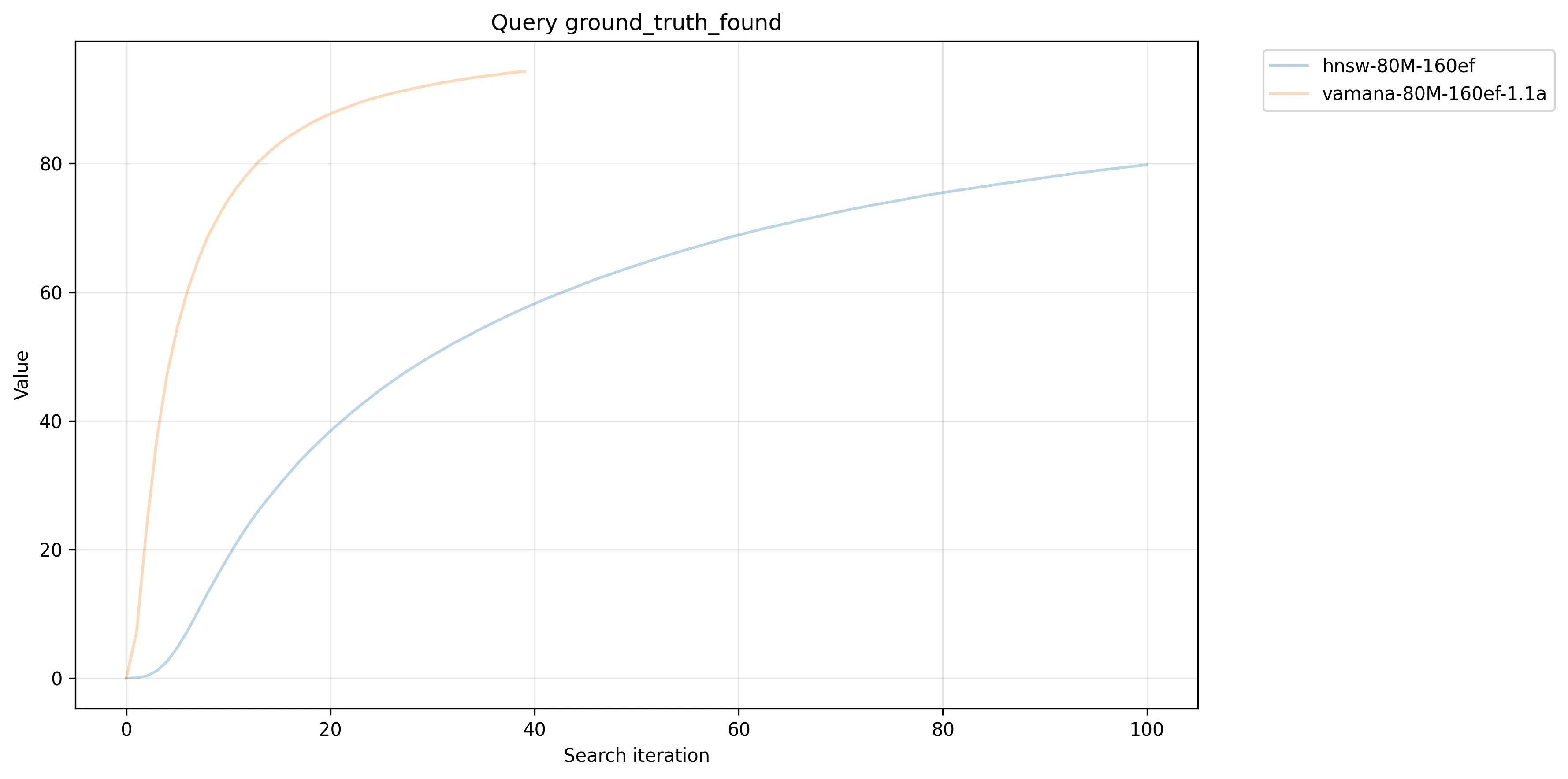
RobustPrune does seem to accomplish both optimization for disk (avoiding tail latencies) while producing higher quality edges.
After flattening, it's possible to use GreedySearch and RobustPrune from Vamana to search and insert into an existing HNSW index. In fact, using GreedySearch often exceeds the accuracy of HNSW on the HNSW index while taking similar time. To do this, I ported relevant parts of hnswlib to hnswlib-rs in order to extract its built graph.
A nice benefit of this is that it's possible to migrate your existing built in-memory HNSW indices to CoreNN cheaply. As we've seen, the graph would not be as optimized as one built from scratch using CoreNN, but as you insert vectors, the graph will optimize over time. This allows you to migrate from in-memory indices and use disk-based scalability, without an expensive reindex and rebuild process.
Similarly, because Vamana tends to outperform HNSW algorithmically, CoreNN also has an ephemeral in-memory mode, to replace the need for HNSW in those situations too.
CoreNN
In the next post, I'll discuss the CoreNN project that puts DiskANN into practice with some improvements on top and the learnings discussed to build an open source vector database that can scale from 1 to 1 billion vectors.